Bayesian Networks

I’ve found the concept of causal models as described in e.g. Pearl’s Causality 2009 to be a very useful tool for statistical thinking. This is the beginning of a series of posts introducing the concept and its applicability.

First, we’ll introduce Bayesian networks (BN). A Bayesian network contains a set of random variables along with a network structure or diagram, a directed acyclic graph showing how the variables are related, and model parameters that specify precisely how variables relate to their neighbors.

Our focus will mainly be on Gaussian Bayesian networks (GBN), that is, Bayesian networks where the variables are jointly a multivariate normal distribution (MVN). Each variable in a GBN is a normal distribution, and they relate to their neighbors as linear regression models.

R has an excellent library for working with these models: bnlearn. We’ll use it to be able to work with these concepts more concretely, but I don’t necessarily recommend using it when more standard methods would suffice. My main goal is to develop thinking tools that are useful in interpreting other models.

Let’s dive in.

library(bnlearn)

mdl.A <- model2network('[X][Y|X]')
mdl.B <- model2network('[X|Y][Y]')
mdl.C <- model2network('[X][Y]')
par(mfrow=c(1, 3))
plot(mdl.A, main='A')
plot(mdl.B, main='B')
plot(mdl.C, main='C')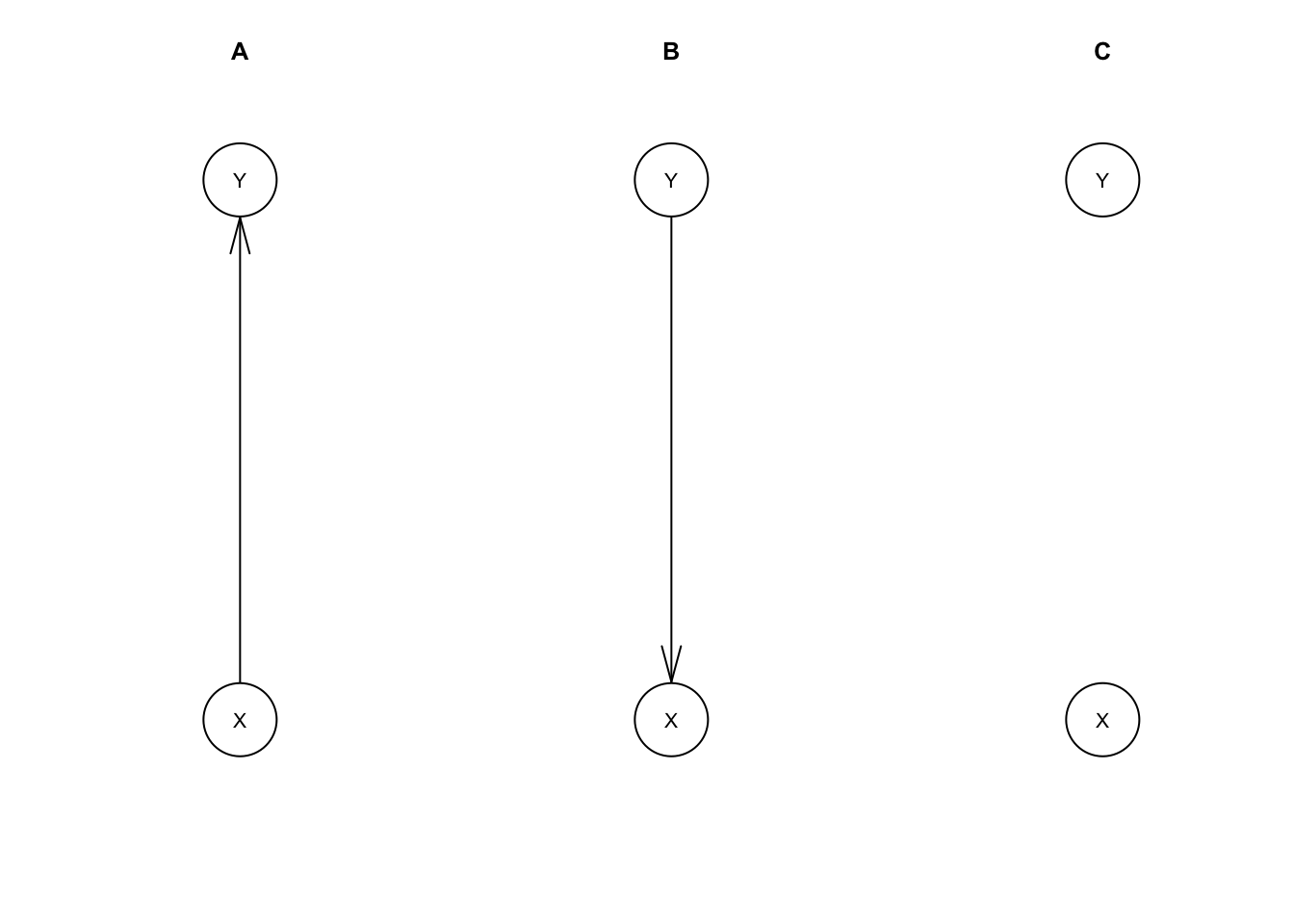

A, B, and C represent all possible network structures for a model with two variables. We’ve left the model parameters unspecified so far. We could specify these manually, but usually we would estimate these from data instead.

The function rmvnorm from the package mvtnorm generates samples from a multivariate normal distribution given a mean vector and covariance matrix. We’ll use that for our working data set.

library(mvtnorm) # for multivariate normal distributions

set.seed(525)
n <- 1000
mu <- c(100, 4+2/3)                 # mean vector
Sigma <- matrix(c(15^2, 3+3/4,      # covariance matrix
                   3+3/4, 1+1/16),
                 nrow=2)
XY <- rmvnorm(n, mu, Sigma)
data.XY <- data.frame(XY)
names(data.XY) <- c('X', 'Y')

For this example, we’ll take X to be a person’s IQ and Y to be a person’s log income. Accordingly we have a mean of 100 and standard deviation of 15 for the distribution of IQ. After undoing the log transformation with \(10^Y\), our income quartiles (25th, 50th, 75th percentiles) are $9,363, $46,416, $230,099.

Let’s fit our models with this data.

fit.A <- bn.fit(mdl.A, data.XY)
fit.B <- bn.fit(mdl.B, data.XY)
fit.C <- bn.fit(mdl.C, data.XY)

fit.A

## 
##   Bayesian network parameters
## 
##   Parameters of node X (Gaussian distribution)
## 
## Conditional density: X
## Coefficients:
## (Intercept)  
##    100.3246  
## Standard deviation of the residuals: 14.95598 
## 
##   Parameters of node Y (Gaussian distribution)
## 
## Conditional density: Y | X
## Coefficients:
## (Intercept)            X  
##  3.00882787   0.01667759  
## Standard deviation of the residuals: 1.005616

Our fitted BN resembles a set of fitted linear regression models, and this isn’t a coincidence. bn.fit assumes you want a GBN if you give it continuous data, so it fit each variable with a linear regression.

fit.A.X <- lm(X ~ 1, data.XY) # Only fitting intercept, effectively just taking the mean
fit.A.Y <- lm(Y ~ X, data.XY)

coef(fit.A.X)

## (Intercept) 
##    100.3246

sd(resid(fit.A.X))

## [1] 14.95598

coef(fit.A.Y)

## (Intercept)           X 
##  3.00882787  0.01667759

sd(resid(fit.A.Y))

## [1] 1.005112

Specifically, each variable is fit as a dependent variable with all of its parents in the network as independent variables. If there are no parents we fit an intercept-only linear regression, which is the same as just taking the mean.

B has the edge between X and Y reversed, so the regressions are reversed too.

fit.B

## 
##   Bayesian network parameters
## 
##   Parameters of node X (Gaussian distribution)
## 
## Conditional density: X | Y
## Coefficients:
## (Intercept)            Y  
##   84.038697     3.478402  
## Standard deviation of the residuals: 14.52296 
## 
##   Parameters of node Y (Gaussian distribution)
## 
## Conditional density: Y
## Coefficients:
## (Intercept)  
##       4.682  
## Standard deviation of the residuals: 1.035599

It may look different, but model B has the same joint distribution for X and Y as A does.

It may also look a bit strange to you. We have an intuition that IQ is determined first and has at least some influence on a person’s income. We would usually have IQ as the independent variable and income as the dependent variable in linear regressions, and the same practice makes sense here. That is, it’s more natural for arrows in a diagram to point from cause to effect. Future posts will discuss this point further.

C is different from A and B. It has a built-in assumption that X and Y are independent; \(X \perp\!\!\!\perp Y\). So, it just fits the marginal distributions for X and Y. We know how we generated our data so we know in advance this won’t fit as well in this case.

Since A and B can model the same set of possible distributions, we say they are observationally equivalent. C can only fit the subset of distributions for which \(X \perp\!\!\!\perp Y\), so C is not observationally equivalent to A and B.

In the next post, we’ll extend Bayesian networks so that the arrows represent causal assumptions about variables in the model.