Natural Experiments and Instrumental Variables Estimation
Now we consider the problem of measuring the strength of causal effects in the presence of confounding variables. As an example, let X be whether a person is a veteran and Y be their income.
It’s easy to compute the correlation between X and Y, but we’re specifically interested in the portion of that correlation that is from the causal effect of X on Y.
To put it more formally, we’re interested in the difference in the expected value of Y if we were to intervene and force someone to participate in a war vs if we were to force them not to. We’ll call this \(\alpha\). \[\alpha = E[Y\,|\,do(X=1)]-E[Y\,|\,do(X=0)]\]
What we can most easily measure given some observational data is the difference in expected value of Y between the groups of people who happened to participate in a war or not in our data. This is exactly the regression coefficient if we were to do a linear regression of Y vs just X. \[r_{YX} = E[Y\,|\,X=1]-E[Y\,|\,X=0]\]
Without any confounders, \(\alpha = r_{YX}\). However, this is not in general the case if we do have confounders.
Let L represent all latent confounding variables, i.e. all variables that have a causal effect on both X and Y. If we can measure L, perhaps if something such as their parents’ income is the only confounder, we can include that in a regression and thereby adequately adjust for it.
library(bnlearn)
library(ggplot2)
library(tidyr)
## Loading required namespace: Rgraphviz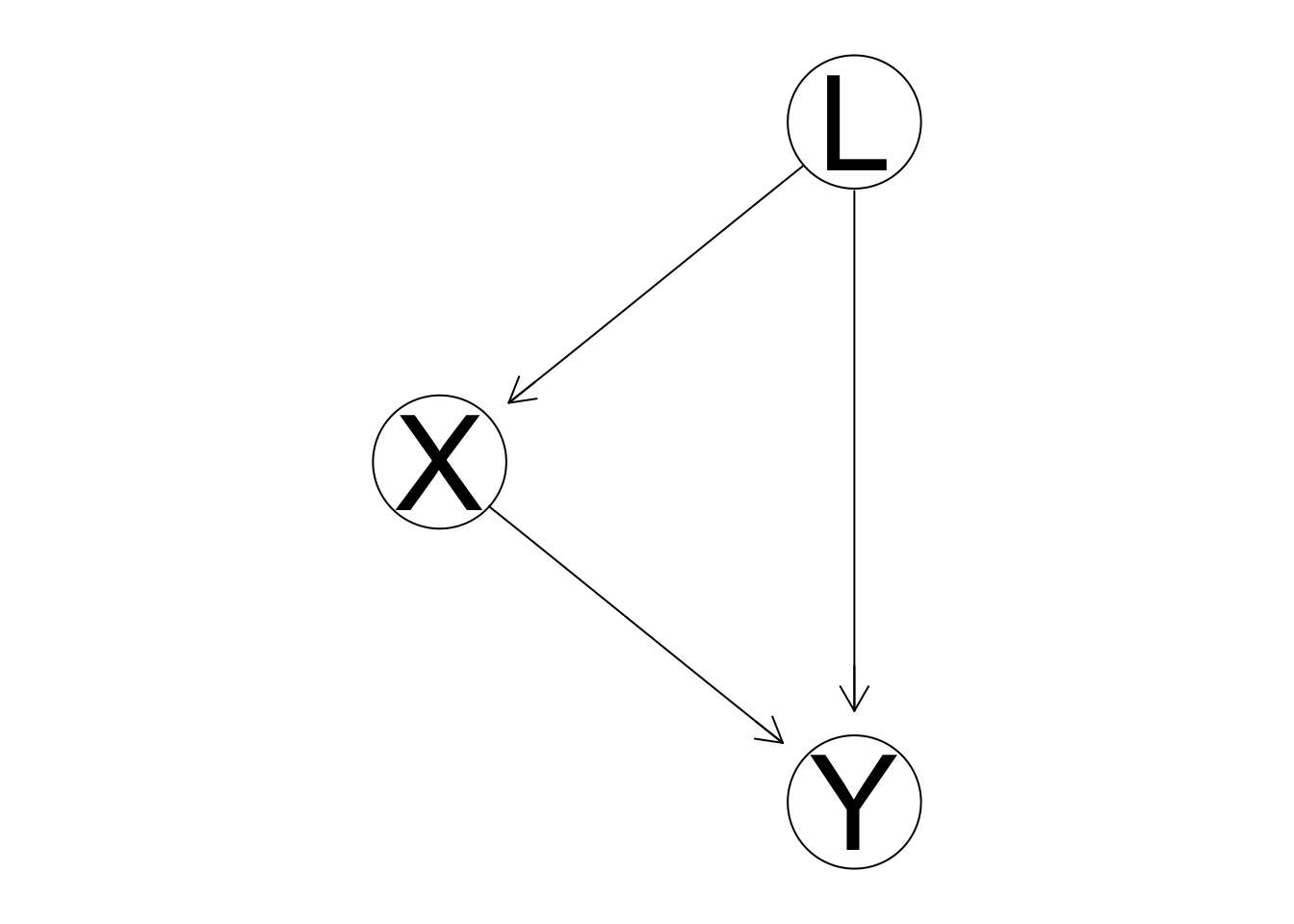
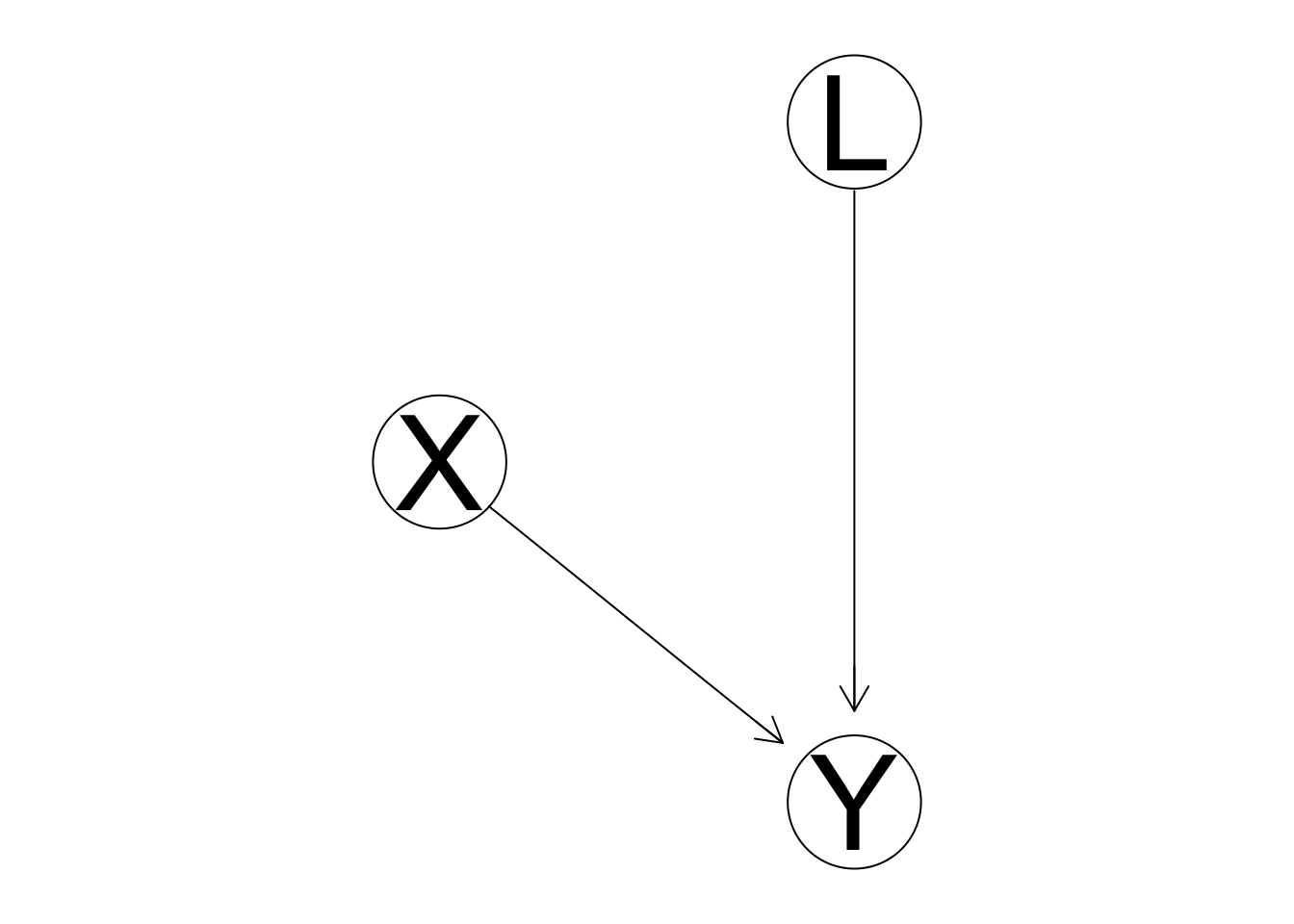
Typically, it isn’t so easy to adjust for confounders. There can be many. We have a couple options. We could find as many possible confounders as we can, adjust for them, and hope that’s enough. Another option is the gold standard in science: experimentation. One can think of an experiment as a direct measurement of the effect of intervention. Graphically, an intervention on X would sever the connection between L and X. L can no longer act as a confounder, and \(\alpha\) can be measured from the experimental data.
For a more realistic model, we can consider that there’s a distinction between telling someone to go to war (putting them in the experimental group) and them actually going to war. Let Z repesent the experimental group a subject is assigned to.
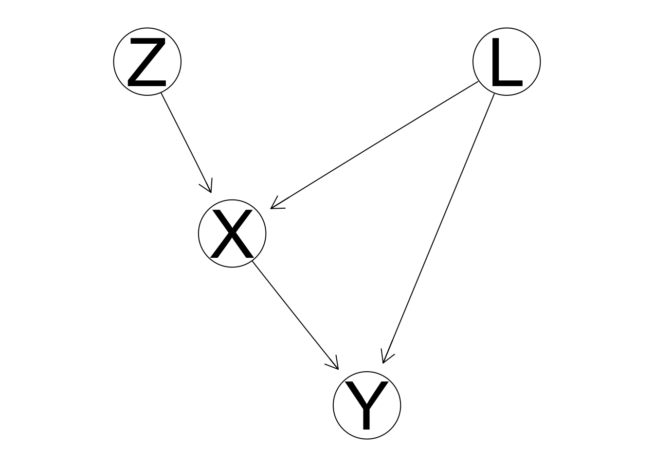
In the context of clinical trials, subjects neglecting to take the medication they were assigned is termed noncompliance. Since there can be a correlation between a subject’s noncompliance and the outcome, our experiment weakens the causal connection between X and L but it isn’t fully eliminated. The relationship between Z and Y is a good approximation to the relationship between X and Y to the extent that noncompliance can be kept low.
For this reason, clinical trials often report the effect of the intent-to-treat (Z) rather than the effect of the treatment itself (X). This can actually result in a more accurate generalization to a doctor’s intent to treat via prescribing a medication, although rates of noncompliance may differ in clinical trials vs clinical practice. So, it would be more ideal if we could measure and use the effect of X itself.
Back to our example of veteran status vs income, another problem we face is that our proposed experiment is unethical. Our desire to learn about the impact of veteran status on future income is not a good reason to ask or force anyone to join the military. However…
We have forced people into the military in the past, with drafts. This process is even randomized. Intent to perform an experiment is irrelevant, randomized assignment with reasonably low noncompliance is sufficient to measure the effect of intervention. We would call such an assignment a natural experiment.
Instrumental variables estimation
Now we’ll discuss a method, instrumental variables estimation, for adjusting for strong noncompliance-like effects, whether we see them in natural or “artificial” experiments.
For an example, I’ll use a simplified, simulated version of a study on the effect of (compulsory) school attendance on income that used instrumental variables estimation. (Angrist et al. 1991)1
We’ll let our X be the number of years someone spent in school and Y be their income. L represents all confounders as usual. Our Z (termed the instrumental variable) will be the person’s birthday(!).
The effect of Z on years in school is from differences is number of compulsory school years from quirks in that regulation. In the data used in the study, students are required to begin school in fall of the calendar year that they turn six. They’re required to remain in school until their sixteenth birthday. They can then drop out of school immediately if they want, even if it’s in the middle of the school year.
Their age when they can leave school is fixed (exactly 16 years), but the age that they’re required to begin school varies with a discontinuous change between a birthday of December 31st and January 1st.
For our simplified model, let’s suppose that how long a student wants to remain in school is normally distributed. If this is less than the time that they’re required to be in school, they wait until their 16th birthday and drop out immediately.
set.seed(52)

nStudent <- 1000000
nDisplay <- 1000

fall.semester <- 3/4

latent <- rnorm(nStudent, 0, 1)

desired.schooling <- 13 + 3*latent + rnorm(nStudent, 0, 0.1)
birthday <- runif(nStudent, 0, 365)/365
min.schooling <- 10 + birthday - fall.semester
actual.schooling <- pmax(desired.schooling, min.schooling) + rnorm(nStudent, 0, 0.2)
In effect, some of the probability density on the lower tail of desired schooling is pushed to the right by a variable amount depending on the student’s birthday.
agg <- gather(data.frame(desired.schooling, actual.schooling))

ggplot(agg) +
  geom_density(aes(value, fill = key), alpha=0.2)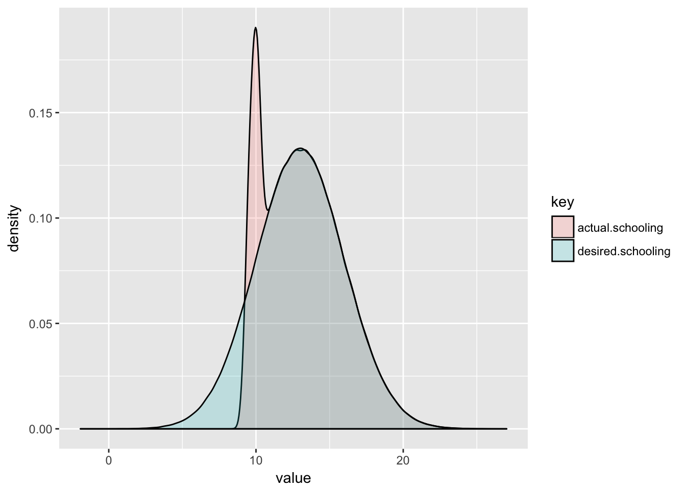
Now we compute the students’ log income. This depends partly on the years they spend in school and partly on the confounding latent variable (plus some random noise). You can see the \(\alpha = 0.1\) coefficient on schooling that we’ll try to measure from the data.
alpha <- 0.1
log.wages <- 6 + alpha*actual.schooling + 0.2*latent + rnorm(nStudent, 0, 0.1)
wages.vs.schooling <- lm(log.wages ~ actual.schooling)
summary(wages.vs.schooling)$coefficients## Estimate Std. Error t value Pr(>|t|)
## (Intercept) 5.0324147 5.625840e-04 8945.179 0
## actual.schooling 0.1731975 4.174565e-05 4148.875 0A regression between log income and years in school gives us \(r_{YX} =\) 0.1731975 \(\neq \alpha = 0.1\). Confounding biases our estimate here.
Let’s say \(\beta = r_{XZ}\) is the regression coefficient for years in school(X) vs a student’s birthday(Z) (in fraction of a full year from January 1st).
schooling.vs.birthday <- lm(actual.schooling ~ birthday)
beta.hat <- coef(schooling.vs.birthday)['birthday']
beta.hat
## birthday
## 0.1450481Now for the key step. We measure the relationship between birthday(Z) and log income(Y). We can assume years in school(X) is the sole intermediate cause between Z and Y. We can also assume that birthdays are determined totally randomly and therefore have no confounding common causes with income. Then the regression coefficient for Y vs Z is \(r_{YZ} = \beta\alpha\).
wages.vs.birthday <- lm(log.wages ~ birthday)
beta.alpha.hat <- coef(wages.vs.birthday)['birthday']
beta.alpha.hat
## birthday
## 0.01456712Our instrumental variables estimate of \(\alpha = 0.1\) is then simply: \(\hat{\alpha} = \frac{\hat{\beta}\hat{\alpha}}{\hat{\beta}} =\) 0.0145671/0.1450481. \(=\) 0.1004295. This is close to the true value.
Angrist, Joshua D., and Alan B. Keueger. “Does compulsory school attendance affect schooling and earnings?.” The Quarterly Journal of Economics 106.4 (1991): 979-1014.↩