Intermediate and Common Causes

We’ll continue with our example of the relationship between IQ (X) and income (Y). We’ll set aside models B (income causes IQ) and C (no relationship) and compare our model A (IQ causes income) with two new models D and E that include a third variable of years in school (Z).

Let’s go straight to graphing these new models.

library(bnlearn)

mdl.A <- model2network('[X][Y|X]')
mdl.D <- model2network('[X][Y|Z][Z|X]')
mdl.E <- model2network('[X|Z][Y|Z][Z]')
par(mfrow=c(1, 3))
plot(mdl.A, main='A')
plot(mdl.D, main='D')
plot(mdl.E, main='E')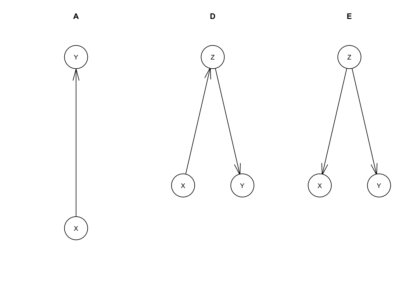

To quickly summarize these models:

A: IQ(X) has a causal effect on income(Y), with no more detail about the mechanism by which this happens
D: IQ(X) has a causal effect on income(Y) entirely because IQ(X) affects years in school(Z) which affects income(Y)
E: IQ(X) does not have a causal effect on income(Y), instead years in school(Z) affects both IQ(X) and income(Y)

These are all observationally equivalent with eadch other if only X and Y are measured. D and E are observationally equivalent even if we include Z.

For model D, the variable Z is called an intermediate cause. D’s causal assertions are compatible with A’s. Model D still implicitly asserts that X has a causal effect on Y, but provides more detail on how that effect works.

Model E’s Z is a common cause or confounder. E serves as an alternative explanation to the correlation between X and Y. Despite being observationally equivalent to model A, E is not causally compatible. E asserts that there is no causal relationship between X and Y.

To help understand how these behave, let’s simulate some data from these networks.

First, D.

set.seed(434)
n <- 10000

X.D <- rnorm(n, 100, 15)
Z.D <- 2*X.D/15 + rnorm(n, 0, 1)
Y.D <- 4 + Z.D/8 + rnorm(n, 0, sqrt(63/64))
#
mu.D <- sapply(list(X.D=X.D, Y.D=Y.D, Z.D=Z.D), mean)
cov.D <- cov(cbind(X.D, Y.D, Z.D))

mu.D  # mean vector

##       X.D       Y.D       Z.D 
## 99.513533  5.677131 13.268614

cov.D # covariance matrix

##            X.D       Y.D        Z.D
## X.D 222.040217 3.8499338 29.7299267
## Y.D   3.849934 1.0623771  0.6380577
## Z.D  29.729927 0.6380577  4.9667985

You can compare the means and covariances with what I used to generate data from an MVN in the first post of this series, Bayesian Networks. You’ll find that X and Y have the same means and covariances, accounting for some noise from our random sample.

Let’s say we’re studying the relationship between IQ and income by analyzing this data. We can reason from prior knowledge that IQ doesn’t change much after childhood and start with a working theory that income in adulthood doesn’t have any effect on IQ. We could hypothesize then, that a correlation between IQ and income would be due to a causal effect from IQ to income, e.g. model A.

We can run a linear regression predicting log income from IQ:

summary(lm(Y.D ~ X.D))

## 
## Call:
## lm(formula = Y.D ~ X.D)
## 
## Residuals:
##     Min      1Q  Median      3Q     Max 
## -3.7165 -0.6649  0.0013  0.6661  4.4179 
## 
## Coefficients:
##              Estimate Std. Error t value Pr(>|t|)    
## (Intercept) 3.9516752  0.0673863   58.64   <2e-16 ***
## X.D         0.0173389  0.0006697   25.89   <2e-16 ***
## ---
## Signif. codes:  0 '***' 0.001 '**' 0.01 '*' 0.05 '.' 0.1 ' ' 1
## 
## Residual standard error: 0.9979 on 9998 degrees of freedom
## Multiple R-squared:  0.06283,    Adjusted R-squared:  0.06274 
## F-statistic: 670.3 on 1 and 9998 DF,  p-value: < 2.2e-16

As expeceted, we get a statistically significant regression coefficient on X.D roughly matching model A (e.g. \(\frac{1}{60}\)).

As anyone should in a regression analysis, we next look for more relevant covariates we can add. Let’s pick years of schooling (Z).

summary(lm(Y.D ~ X.D + Z.D))

## 
## Call:
## lm(formula = Y.D ~ X.D + Z.D)
## 
## Residuals:
##     Min      1Q  Median      3Q     Max 
## -3.6327 -0.6477 -0.0090  0.6566  4.4762 
## 
## Coefficients:
##              Estimate Std. Error t value Pr(>|t|)    
## (Intercept) 3.9585966  0.0668744  59.194   <2e-16 ***
## X.D         0.0006962  0.0014915   0.467    0.641    
## Z.D         0.1242975  0.0099723  12.464   <2e-16 ***
## ---
## Signif. codes:  0 '***' 0.001 '**' 0.01 '*' 0.05 '.' 0.1 ' ' 1
## 
## Residual standard error: 0.9902 on 9997 degrees of freedom
## Multiple R-squared:  0.07718,    Adjusted R-squared:  0.07699 
## F-statistic:   418 on 2 and 9997 DF,  p-value: < 2.2e-16

Now this matches what we see for Y.D in our code above. The coefficient for Z.D is roughly \(\frac{1}{8}\) and the coefficient for X.D is near zero and statistically insignificant.

We saw a correlation between X and Y without Z in our regression, but did not see this when we included Z. What’s going on exactly?

The regression coefficient for X here has a very specific meaning. It’s the relationship between X and Y if we adjust for Z. In other words, if we break Z up into groups (e.g. high school graduates, bachelors, masters, PhD) and regress X and Y within each group, what relationship do we see?

The assumption built into this model is that all of the causal effect from X to Y is through Z. i.e. Z is the sole intermediate cause between X and Y. So of course, once we’ve accounted for Z, learning X gives us no more information about Y.

Phrasing this differently, X is dependent on Y, \(X \perp\!\!\not\!\perp Y\), but X is conditionally independent of Y given Z, \(X \perp\!\!\!\perp Y\,|\,Z\). This is a key fact about the model, as that conditional independence is the only constraint on the joint distribution of X, Y, and Z.

This conditional relationship given Z is not necessarily the most important relationship. There still really is a causal relationship between X and Y. If that causal relationship is what we wanted to measure, adding Z to our regression was the wrong thing to do. There’s a common misconception that adding more covariates to a regression either helps, does nothing, or only hurts a little by adding noise to our estimates. That is true for pure prediction applications, but for causal inference this serves as a counterexample.

And, let’s look into E.

set.seed(300)
n <- 10000
#
Z.E <- rnorm(n, 13+1/3, sqrt(5))
X.E <- 20 + 6*Z.E + rnorm(n, 0, sqrt(45))
Y.E <- 4 + Z.E/8 + rnorm(n, 0, sqrt(63/64))
#
mu.E <- sapply(list(X.E=X.E, Y.E=Y.E, Z.E=Z.E), mean)
cov.E <- cov(cbind(X.E, Y.E, Z.E))

mu.E

##        X.E        Y.E        Z.E 
## 100.106010   5.658646  13.358268

cov.E

##            X.E       Y.E        Z.E
## X.E 228.705196 4.0476436 30.7851587
## Y.E   4.047644 1.0923873  0.6611757
## Z.E  30.785159 0.6611757  5.1291326

The joint distribution for X, Y, and Z is the same as with C, so our regressions will give essentially the same results (you can check this if you like). However, the causal assumptions behind them are no longer true. There is no causal relationship between X and Y. The correlation we nonetheless see between them is due to the common cause variable Z.

Here, including Z in the regression shows the true causal effect between X and Y, i.e. zero correlation.

Let’s briefly introduce two more models F and G, just to contrast them with D and E. These include a direct link between X and Y in addition to the connection through the third variable Z.

mdl.F <- model2network('[X][Y|X:Z][Z|X]')
mdl.G <- model2network('[X|Z][Y|X:Z][Z]')
par(mfrow=c(1, 2))
plot(mdl.F, main='F')
plot(mdl.G, main='G')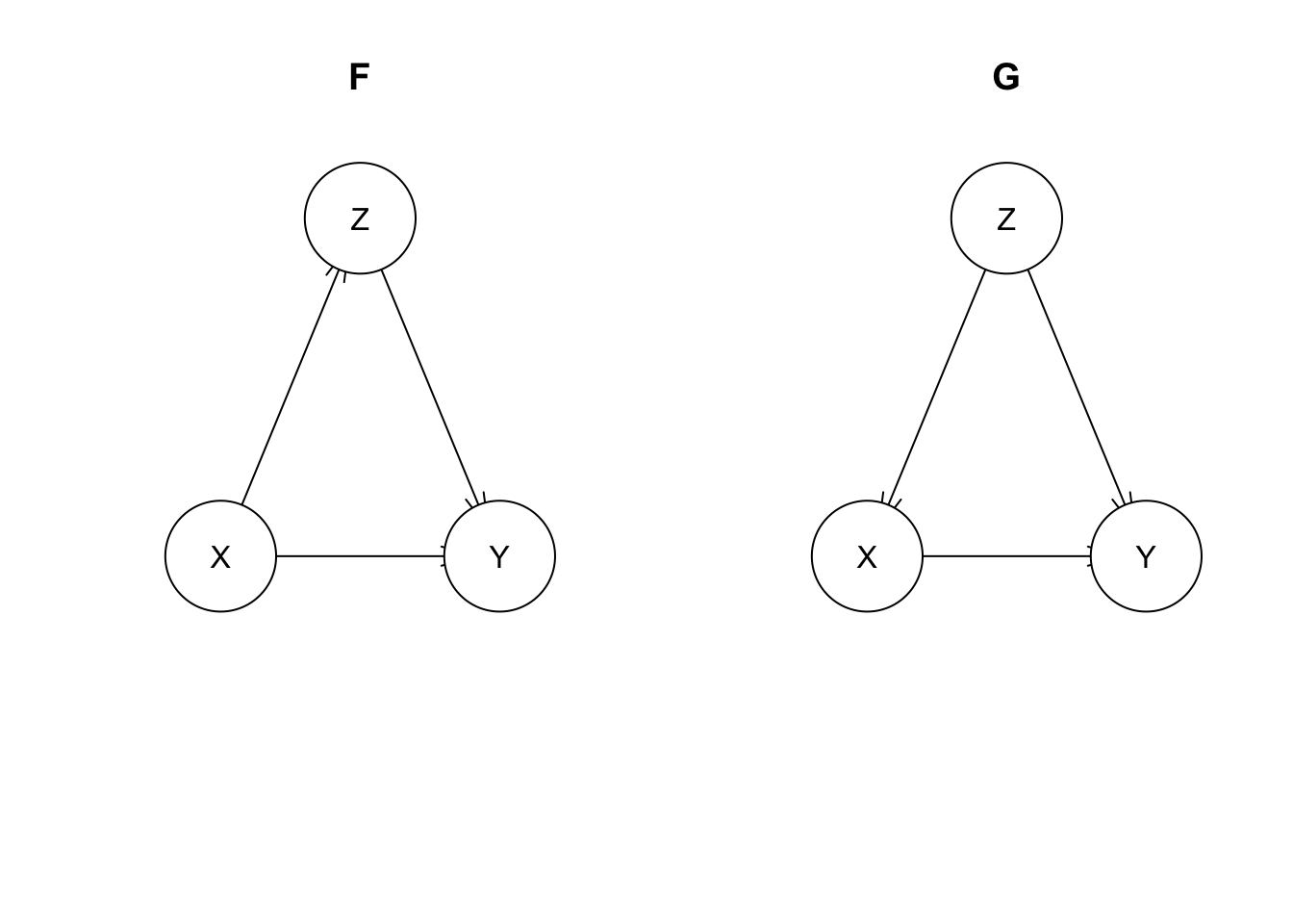

And, let’s simulate some data from F. (G will have different code, but can generate the same distribution)

set.seed(63)
n <- 1000000 # pumping up the sample size this time. Z has a weak effect on Y, and we'll try to detect that
#
X.F <- rnorm(n, 100, 15)
Z.F <- 2*X.F/15 + rnorm(n, 0, 1)
Y.F <- 4 + X.F/64 + Z.F/128 + rnorm(n, 0, sqrt(63/64))
#
mu.F <- sapply(list(X.F=X.F, Y.F=Y.F, Z.F=Z.F), mean)
cov.F <- cov(cbind(X.F, Y.F, Z.F))

mu.F

##       X.F       Y.F       Z.F 
## 99.992559  5.665259 13.332106

cov.F

##            X.F       Y.F        Z.F
## X.F 224.622847 3.7337616 29.9331900
## Y.F   3.733762 1.0479060  0.5028429
## Z.F  29.933190 0.5028429  4.9895325

You can see from the means/covariances of X/Y that this is observationally equivalent to model A (exlucing Z). However, \(\mathrm{cov}_F(Y, Z) \neq \mathrm{cov}_D(Y, Z)\). It’s hard to see, but cov.F[2, 3] \(=\) 0.5028429 \(\neq\) cov.D[2, 3] \(=\) 0.6380577. This isn’t conclusive proof that they’re different as it may just be noise, but you can verify this with a sufficiently large sample size or analytically.

If we look at the regression of Y vs X and Z, we get:

summary(lm(Y.F ~ X.F + Z.F))

## 
## Call:
## lm(formula = Y.F ~ X.F + Z.F)
## 
## Residuals:
##     Min      1Q  Median      3Q     Max 
## -4.9304 -0.6699  0.0002  0.6711  4.5347 
## 
## Coefficients:
##              Estimate Std. Error t value Pr(>|t|)    
## (Intercept) 4.0031089  0.0066983 597.632  < 2e-16 ***
## X.F         0.0159188  0.0001479 107.609  < 2e-16 ***
## Z.F         0.0052793  0.0009926   5.319 1.04e-07 ***
## ---
## Signif. codes:  0 '***' 0.001 '**' 0.01 '*' 0.05 '.' 0.1 ' ' 1
## 
## Residual standard error: 0.9929 on 999997 degrees of freedom
## Multiple R-squared:  0.05925,    Adjusted R-squared:  0.05925 
## F-statistic: 3.149e+04 on 2 and 999997 DF,  p-value: < 2.2e-16

This time, we see that X.F has a statistically significant regression coefficient. That means \(X \perp\!\!\not\!\perp Y\,|\,Z\), unlike with models D and E. Z only partially explains the effect of X on Y.

Learning causal structure

bnlearn has functionality for automatically learning causal structure from data. The package includes several algorithms. gs (the Grow-Shrink algorithm) works on similar principles as we’ve been discussing in this post. It essentially does a sequence of (multiple) linear regressions and checks the statistical significance of the coefficients to determine (conditional) independence relationships.

You’ll find this functionality to be quite finicky, even in toy problems. I wouldn’t say this has much practical use, but it is still useful to understand as the problem these algorithms face is essentially the same as for anyone attempting causal inference.

Let’s try this on model E, but leaving Z out.

bn.E.X.Y <- gs(data.frame(X=X.E, Y=Y.E))
plot(bn.E.X.Y)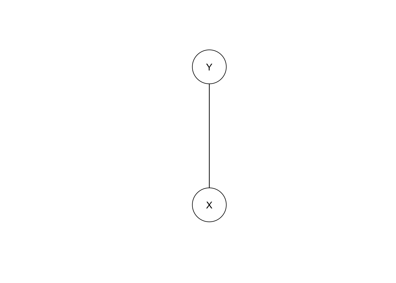

The undirected edge means X causes Y, Y causes X, OR that there’s a hidden common cause. That third case is the reality here.

If we inlude Z:

bn.E.X.Y.Z <- gs(data.frame(X=X.E, Y=Y.E, Z=Z.E))
plot(bn.E.X.Y.Z)

This is compatible with model D, so gs can’t distinguish these models. i.e. they’re observationally equivalent.

Finally, gs on model F gives:

bn.F.X.Y.Z <- gs(data.frame(X=X.F, Y=Y.F, Z=Z.F))
plot(bn.F.X.Y.Z)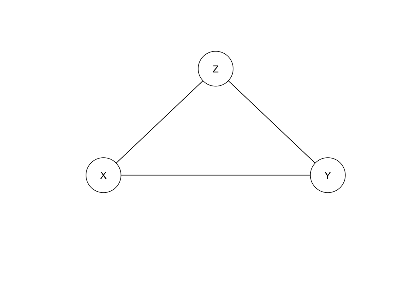

So, model F is indistinguishable from model G.

Next we’ll look at common effects.